- 83 views
While discussing the valuations of markets in general and stocks in particular, the most commonly used tool is undeniably a Price Earnings multiple (PE multiple). A PE multiple is a short-hand for the valuation process — not valuation per se — and no one should fail to make that distinction. The good thing about multiples is that they save time. However, they also incorporate a lot of economic assumptions that need to be unpacked for investors for them to accurately understand their meaning.
Dissecting the earnings multiple
Let us first dissect and simplify the formula for P/E into three easily understandable vectors:
| 𝑃/𝐸 = | 𝑅𝑜𝐸−𝑔 |
| {𝑅𝑜𝐸 𝑋 (𝐶𝑜𝐸−𝑔)} |
While RoE is the Return on Equity, CoE is the Cost of Equity and g is the Earnings Growth. As is evident, PE multiple has a direct relationship with both RoE and growth and an inverse relationship with CoE.
Annexure 1 provides the detailed working of the above equation
Let’s look at the following table to comprehend the right level of PE multiples for businesses at varying levels of RoE as well as growth rates. We have assumed that the Cost of Equity is 12% and that the levels of RoE and growth rates are steady and sustainable.
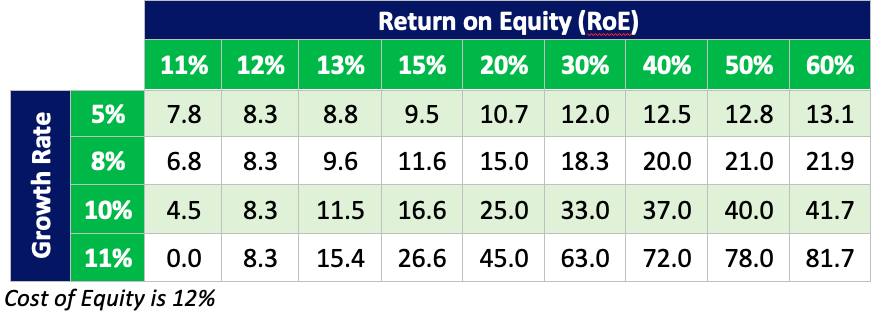
What this clearly proves is that different businesses ought to be trading at very different levels of PE multiples on account of their outcomes in terms of growth and RoEs. At one extreme we have businesses like Nestle that have an average RoE higher than 60% and a sustainable growth of 11%, thereby commanding a very high valuation. At the other extreme, we have businesses like NTPC that have a RoE of around 12% and sustainable growth of 10% or lower, which command a low valuation.
Key takeaways from the table:
- Companies, which have RoEs lower than the cost of capital, destroy value if they grow faster. This is the only group that witnesses PE derating with growth increasing. Therefore, such businesses should stop growing immediately and first fix their profitability if they must create any value for their shareholders.
- Companies that have their RoEs equal to their cost of capital are just stationary in terms of their multiple. It does not matter whether they grow fast or slow, as their multiples would remain the same.
- If both RoE and growth or either of the two improves or deteriorates for good, then the business will witness a sustainable improvement or deterioration in multiples.
- For companies that have a low RoE, an increase in growth leads to a rerating, albeit at a slower rate. But for companies that have a high RoE, any acceleration in growth can lead to an exponential increase in multiples.
- For companies that have a low rate of growth, incremental improvement in RoEs leads to a slower rerating, while those at a higher rate of sustainable growth witness a higher growth in multiples as RoEs move up.
- If a company is operating at higher than cost of capital, then regardless of its level of growth rates or RoEs, incremental change in growth moves the valuation faster than incremental change in RoEs.
The most important message that we can draw from the calculations in the above table is that no level of PE should be judged as too high or too low without appreciating its drivers. Businesses that have competitive advantages leading to winning business models and therefore high RoEs as well as strong growth, will trade at high multiples. Remember that multiples are just short-hand for an intrinsic value exercise.
The sustainability of quality and the growth of a franchise and hence the compounding impact of it over decades can only be captured by doing an intrinsic value exercise like a DCF. Such compounding can never be appreciated by looking at valuation multiples, which are unable to look beyond the next one or two years and hence look expensive from a near-term perspective, although they may not actually be so.
The converse of this is also true. If a business has a weak franchise that lacks pricing power and is unable to generate strong RoEs or if it is unable to grow at a respectable rate or both, it will trade at a poor multiple. While one may get attracted towards these multiples and hope to play a rerating of these, such businesses may already be trading at the valuations that are warranted.
Earnings multiple as a tool for comparison
Now that we are sufficiently clear with what leads to these multiples, let us try to understand the obvious mistakes that one makes while using them in everyday analysis.
The most obvious one is comparing PEs across different industries. This can be grossly incorrect as the return profile and sustainability of growth can be vastly different amongst industries. For example, it is surprising when investors talk about consumer staples sector to be very expensive in comparison to the Indian pharma industry. For similar levels of future growth outlook, the consumer staples sector ought to be trading at a higher valuation because of its significantly better RoEs.
For instance, Marico rightfully trades at a significantly higher multiple than Cipla, although both would have a similar growth profile as Marico’s RoEs are almost thrice than that of Cipla’s (10-year average of 35% vs 13%).
In fact, comparing PE ratios within the same industry is also fraught with risks. Depending on the wide moats that some businesses enjoy within an industry — as well as their ability to be more efficient in terms of capital expenditure, working capital and asset turnover — the outcomes in terms of RoEs and therefore PEs can be vastly different. Within the same industry there are always cases of certain businesses growing faster than the overall industry, which should itself be a reason for a higher PE.
For instance, the earnings multiple of Asian Paints is significantly higher than that of Akzo Nobel, both on account of better growth and higher RoE. It would be incorrect to assume that a mean reversion should happen between these two companies in terms of earnings multiple.
Last but by no means the least, comparing the PE of a firm with its own history can also lead to wrong conclusions. For instance, if a company has shown an improving trend in its RoEs then its multiple will also improve. This is indeed the case with many high- quality, deep-moated companies, which are not only able to defend their margins but are also constantly striving to become more efficient and thereby improve their ROCEs. For such companies, looking at the current PE being at a premium to the long-term history may not be correct. And, the reverse is equally true. If a business is either coming down in terms of its growth trajectory or is expected to witness a deterioration in its RoEs, it should trade at a discount to its historic averages.
A perfect case in point here is Page Industries. While Page has always been a strong company, it has become stronger in the last decade compared to the previous decade. Its ever-improving distribution reach and brand recall have led to its moats becoming wider, and as a result, its ROCEs have gone up by about 10-15 percentage points post 2015. This itself led to its multiple moving up, which many investors initially felt was unjustified. But these higher multiples have held up since 2015, ever since improving capital efficiency was baked in by the markets.
Impact of term structure of interest rates on PE
The effect of changes in the expected growth rate on the PE of a firm varies as per the level of interest rates. The PE ratio is more sensitive to changes in expected growth rates when interest rates are low than when they are higher. This is because growth produces cash flows in the future and the present value of these cash flows is smaller at high interest rates. Consequently, the effect of changes in the growth rate on the present value tend to be smaller.
When a firm reports earnings that are significantly higher than expected (a positive surprise) or lower than expected (a negative surprise), investors’ perceptions of the expected growth rate for this firm can change concurrently, leading to a price effect. One should expect to see greater price reactions for a given earnings surprise, positive or negative, in a low-interest rate environment than in a high-interest rate environment. Thus, PE multiples are expected to contract or expand more in low-interest rate environments than in high-interest rate environments.
Let us take an example: At 12% Cost of Equity, the reduction in growth from 10% to 8% for a company with an RoE of 30% will lead to the PE multiple derating by nearly 45%. When CoE moves to 13%, for the same company, the PE derating — on account of growth coming down from 10% to 8% — will be 35%. Likewise at 12% CoE, an increase in growth from 10% to 11% for a company with an RoE of 40% will lead to the PE multiple rerating by about 90%. When CoE moves to 13% for the same company, the PE rerating — on account of growth moving from 10% to 11% — will be about 45%
Conclusion
Although PE ratios are the most commonly used valuation metric, a correct understanding of its constituents is essential. The biggest advantage of a PE multiple is its ease of use as against a Discounted Cashflow exercise, which requires a lot of assumptions and projections. However, one must be aware of the drivers of PE before making a judgement about the ratio being too high or too low for a given firm or a set of firms.
Annexure
Deriving the price earnings multiple equation
P/Es are calculated by deriving a simple model for earnings in terms of the key value drivers from the dividend discount model (DDM). This process is explained below.
The one big assumption made in this exercise is that the company is steady and stable, resulting in its ROE as well as dividend growth being constant. This assumption allows value to be expressed in terms of the first forecast year dividend per share (DPS), long- run prospective growth in DPS (gd) and the cost of equity (COE):
| 𝐹𝑎𝑖𝑟 𝑆ℎ𝑎𝑟𝑒 𝑃𝑟𝑖𝑐𝑒 = | 𝐷𝑃𝑆1 | (Constant growth DDM) |
| (𝐶𝑜𝐸-𝑔d) |
Dividends can be expressed in terms of earnings:
𝐷𝑃𝑆𝑛=𝐸𝑃𝑆𝑛−𝑟𝑒𝑝𝑠𝑛
(𝑟𝑒𝑝𝑠𝑛 represents retained earnings per share)
This can be substituted in the constant growth DDM:
| 𝐹𝑎𝑖𝑟 𝑆ℎ𝑎𝑟𝑒 𝑃𝑟𝑖𝑐𝑒 = | 𝐷(𝐸𝑃𝑆1−𝑟𝑒𝑝𝑠1) |
| (𝐶𝑜𝐸−gd) |
If we assume that ROE is constant over time, i.e., steady state conditions prevail, ‘reps’ can be expressed in terms of earnings, earnings growth and return on equity. The steps to arrive at the appropriate expression for ‘reps’ are given below:
| 𝐸𝑎𝑟𝑛𝑖𝑛𝑔𝑠 𝐺𝑟𝑜𝑤𝑡ℎ = 𝑔𝑒 = | 𝐸𝑃𝑆n+1−𝐸𝑃𝑆𝑛 |
| 𝐸𝑃𝑆n |
(the numerical subscripts denote the year) also;
𝐸𝑃𝑆𝑛=𝑅O𝐸*𝑆𝐻𝐹𝑛−1
(ROE represents return on equity (after tax) and SHF represents shareholders’ funds expressed per share)
Finally, the change in shareholders’ funds will be driven by the retained earnings and therefore can be written as:
𝑆𝐻𝐹𝑛=𝑆𝐻𝐹𝑛−1+ 𝑟𝑒𝑝𝑠n
By substituting the above two equations in the growth equation we get
| 𝑔𝑒 = | [𝑅𝑜𝐸*(𝑆𝐻𝐹𝑛−1+𝑟𝑒𝑝𝑠n)−𝑅O𝐸*𝑆𝐻𝐹𝑛−1] |
| 𝑅O𝐸*𝑆𝐻𝐹n-1 |
This simplifies to:
| 𝑔𝑒 = | 𝑟𝑒𝑝𝑠𝑛 |
| 𝑆𝐻𝐹n-1 |
If 𝑆𝐻𝐹n-1 is expressed in EPS terms we get:
| 𝑔𝑒 = | 𝑟𝑒𝑝𝑠𝑛*𝑅O𝐸 |
| 𝐸𝑃𝑆n |
This can be substituted in the fair share price equation:
| 𝐹𝑎𝑖𝑟 𝑆ℎ𝑎𝑟𝑒 𝑃𝑟𝑖𝑐𝑒 = | 𝐸𝑃𝑆*(𝑅O𝐸−𝑔𝑒) |
| 𝑅O𝐸*(𝐶O𝐸−𝑔𝑒) |
By dividing each side of the equation by the EPS we can establish the fair price earning multiple as:
| 𝐹𝑎𝑖𝑟 𝑃 /𝐸𝑀𝑢𝑙𝑡𝑖𝑝𝑙𝑒 = | 𝑅O𝐸−𝑔𝑒 |
| 𝑅O𝐸*(𝐶O𝐸−𝑔𝑒) |